1. Listening for nuances in musical expression

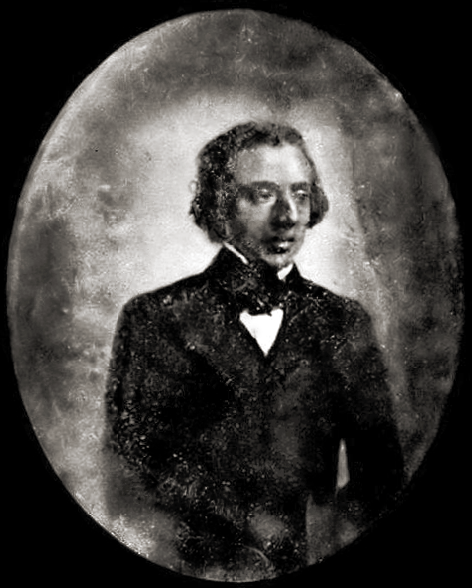
Fryderyk Chopin (1810 - 1849) clearly adored the Mazurka —
he composed more Mazurkas than any other form of music, producing altogether about 60 starting from his teenage years
to the end of his short life. Of these, 45 Mazurkas were published with his approval during his lifetime.

Originally a Polish folk dance, in his solo piano music Chopin elevated the Mazurka to a peak of artistic emotional expression.

He once wrote that his Mazurkas were "not for dancing" [1]. Some are lively while others have a slower tempo. Taking the traditional dance rhythm only as a point of reference or inspiration, he infused them all with his sensitive personal idiom, and above all with żal, a Polish word that Chopin himself used to describe his musical emotional world [2]; it can mean regret, longing, nostalgia, melancholy, grief, and much more.

The Op.63 set of three Mazurkas was the last that he sent out for publication (1847). The final number, Op.63 No.3, is in the key of C-sharp minor, incidentally the same tonality as the Lento con gran espressione of many years earlier. The tempo is marked Allegretto, and the principal theme has the character of a kujawiak [3] (one of the five national dances of Poland) which, compared with the mazur, is typically more calm, slow, songful.

This short piece is structured in three main parts. The first part (bars 1-32) states the main theme. The second part (bars 33-48) is a contrasting episode in the relative major key (D-flat, the enharmonic equivalent of C-sharp); it starts sotto voce (under the breath) and gradually intensifies through harmonic modulations to the third part (bars 49 onwards) where the original theme returns even more poignantly than before. In the final couple of lines (bars 65 onwards) Chopin presents the main theme in a kind of nostalgic duet, the lower voice echoing the upper melody — yet another example of his love for Bach and counterpoint. After all the delicate poignancy, the piece ends with a muscular flourish.

Listen to the following five recordings of this last published Mazurka. The performing artists' names are intentionally not revealed here, to avoid any bias while listening. Please try to ignore any audio imperfections such as differences in overall volume, or surface noise due to old recording technology. Instead, focus your attention on each pianist's expressivity: the way in which Chopin's melodies, harmonies, rhythms, his soul and żal are expressed.

One and the same piece of music; five distinct performances. There are occasional similarities, but even more remarkable are the differences in approach, temperament, emotional expression. Regarding overall duration, these performances range from just under 2 min (fastest) to 2¾ min (slowest). Equally striking are the differences in nuance: the shaping of melodic contours, the articulation of left-hand chords, the ebb-and-flow of the tempo rubato, and the dynamics of certain phrases.

For example at bars 61-62, in the absence of any explicit dynamic marking in the score, one pianist intensifies the phrase by growing louder and faster and abruptly stopping at the rest, while other pianists "intensify" by diametrically opposite means, getting softer, slower, more deliberate.

2. Quantifying expressive deviations in timing

We now take it for granted that a music performance can be easily recorded, saved to a convenient medium, and played back at will. Performers, music teachers, students, and anyone who loves music can easily listen to and compare different recordings, thus greatly enhancing our enjoyment and learning experiences. To complement this subjective or qualitative, auditory impression, music signal processing technology can provide an objective or quantitative perspective, by numerical analyses of the recorded audio.

As mentioned above, one aspect of performance expressivity is how an artist stretches time by slowing down or quickening the pace of music. Such artistic deviations in timing are inherent to most human performances, and have been studied for many years (e.g., [5]), but manual labelling of musical events such as beats or bars takes considerable time and effort, thus limiting the amount of music that can be analyzed. In more recent years, music signal processing techniques such as Chroma feature extraction [6] and Dynamic Time Warping (DTW) [7] have been applied to automatically [8] match the timing of a performance audio with that of an expressionless, dead-pan audio rendered from the score by software. In this way, the performer's expressive deviations from the literal score may be quantified.

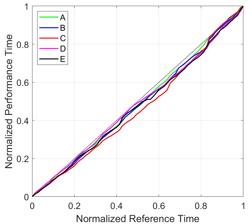
The results of such automated music synchronization analyses of our five recordings of the Chopin Mazurka, are shown in the Time Warping Paths below. The figure on the left shows the raw Warping Paths, where the horizontal axis Reference Time represents the expressionless audio which was rendered at a steady 100 quarter-notes per minute. The different overall slopes of the five curves indicate the different overall durations of the human performances. Additionally, subtle differences in the shape or undulations of each curve are also evident. These local differences in timing can be compared more clearly in the figure on the right, where the overall durations are normalized to a common range and the 45° dashed line represents a dead-pan performance. While each performance begins at the same point (0) and ends at the same point (1), in between we see both commonalities and differences in individual characteristics of the ebb-and-flow of the recorded music's pulse.

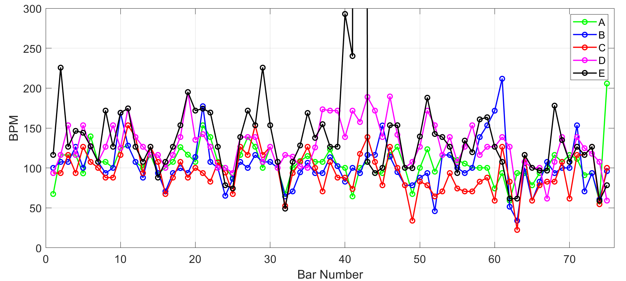
By taking the numerical derivative of these Warping Paths, we obtain the Tempo Curves shown below. These curves show even more clearly that the five artists played this piece with a wide range of local tempi. In the face of such intra- and inter-individual variations, the nominal tempo (e.g., 100 BPM) is nothing more than a rough guide.

While such quantitative data can reveal interesting performance characteristics, one needs to be mindful that the results obtained by such automated techniques can be sensitive to various parameter settings. The current analysis used standard Chroma features with gamma logarithmic compression, extracted at analysis frames of duration 125 ms with a frame shift of no greater than 125 ms, and the DTW distance metric was Euclidean. Modification of any of these or other settings, or use of variant acoustic features, may frustratingly yield somewhat different Warping Paths and Tempo Curves. Even with the current parameter settings, the outlier peaks of over 200 BPM from bar 40 for Recording E seen in the figure above, are most likely errors — while pianist E certainly quickens the tempo in that passage, careful listening reveals the correct value to be about 144 BPM at bar 40 rising to about 190 BPM two bars later.

Perhaps the only sure way to assess the validity of automated analysis results, is to compare them either with manually-determined time-stamps, or those calculated from MIDI data where available. This is an open avenue for further research.

REFERENCES

[1] F. Chopin Chopin's Letters, collected by H. Opienski, translated by E. L. Voynich
(a letter to his family in Warsaw, from Vienna, 22 Dec 1830)
Dover Publications (New York), 1988.
[2] F. Liszt Life of Chopin, translated by M. W. Cook
Dover Publications (New York), 2005.
[4] J. C. Hadden (1903), quoting J. Seligmann who attended the 1848 Glasgow concert Chopin
E. P. Dutton & Co. (New York).
[5] B. Repp (1998) A microcosm of musical expression. I. Quantitative analysis of pianists' timing in the initial measures of Chopin's Etude in E major
J. Acoust. Soc. Am., 104(2), 1085-1100.
[6] T. Fujishima (1999) Realtime chord recognition of musical sound: a system using common lisp music
in Proc. Int. Computer Music Conf., 464-467.
[7] H. Sakoe & S. Chiba (1978) Dynamic programming algorithm optimization for spoken word recognition
IEEE Trans. on Acoust. Speech and Sig. Process., ASSP-26 No.1, 43-49.
[8] M. Müller et al. (2009) Towards automated extraction of tempo parameters from expressive music recordings
in Proc. Int. Music Info. Retrieval (ISMIR) Conf., 69-74.